Generate atrial fibers

This example shows how to generate atrial fibers using the Laplace-Dirichlet Rule-Based (LDRB) method.

Warning

When using a standalone version of the DPF Server, you must accept the license terms. To accept these terms, you can set this environment variable:

import os
os.environ["ANSYS_DPF_ACCEPT_LA"] = "Y"

Perform the required imports

Import the required modules and set relevant paths, including that of the working directory, model, and LS-DYNA executable file. This example uses DEV-104373-g6d20c20aee.

import os
from pathlib import Path

import numpy as np
import pyvista as pv

from ansys.health.heart.examples import get_preprocessed_fullheart
import ansys.health.heart.models as models
from ansys.health.heart.simulator import BaseSimulator, DynaSettings

# Specify the path to the working directory and heart model. The following path assumes
# that a preprocessed model is already available
workdir = Path.home() / "pyansys-heart" / "downloads" / "Rodero2021" / "01" / "FullHeart"

path_to_model, path_to_partinfo, _ = get_preprocessed_fullheart()

# Specify LS-DYNA path
lsdyna_path = r"ls-dyna_smp"

# Load heart model
model: models.FourChamber = models.FourChamber(working_directory=workdir)
model.load_model_from_mesh(path_to_model, path_to_model.replace(".vtu", ".partinfo.json"))

Instantiate the simulator

Instantiate the simulator and modify options as needed.

Note

The DynaSettings object supports several LS-DYNA versions and platforms, including smp, intempi, msmpi, windows, linux, and wsl. Choose the one that works for your setup.

# instantiate LS-DYNA settings of choice
dyna_settings = DynaSettings(
    lsdyna_path=lsdyna_path, dynatype="intelmpi", num_cpus=4, platform="windows"
)

simulator = BaseSimulator(
    model=model,
    dyna_settings=dyna_settings,
    simulation_directory=os.path.join(workdir, "simulation"),
)

simulator.settings.load_defaults()

# remove fiber/sheet information if it already exists
model.mesh.cell_data["fiber"] = np.zeros((model.mesh.n_cells, 3))
model.mesh.cell_data["sheet"] = np.zeros((model.mesh.n_cells, 3))

Compute atrial fibers

# compute left atrium fiber
la = simulator.compute_left_atrial_fiber()

# Appendage apex point should be manually given to compute right atrium fiber
appendage_apex = [39, 29, 98]
ra = simulator.compute_right_atrial_fiber(appendage_apex)

Note

You might need to define an appropriate point for the right atrial appendage. The list specifies the x, y, and z coordinates close to the appendage.

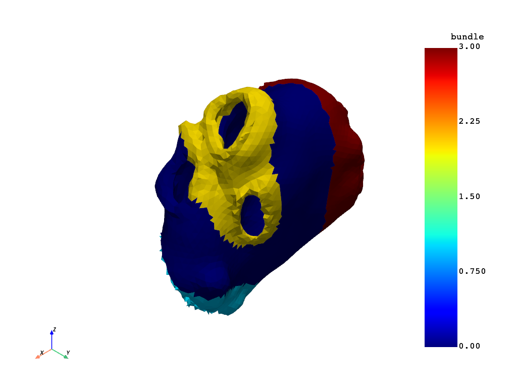
Plot left atrial bundles

la.cell_data["bundle"] = la.cell_data["bundle"].astype(np.int32)
la.set_active_scalars("bundle")
la.plot()

Static Scene

Interactive Scene

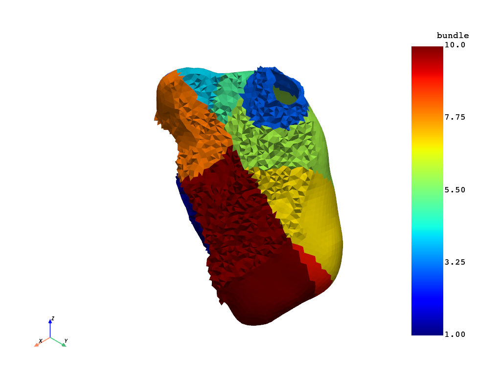
Plot right atrial bundles

ra.cell_data["bundle"] = ra.cell_data["bundle"].astype(np.int32)
ra.set_active_scalars("bundle")
ra.plot()

Static Scene

Interactive Scene

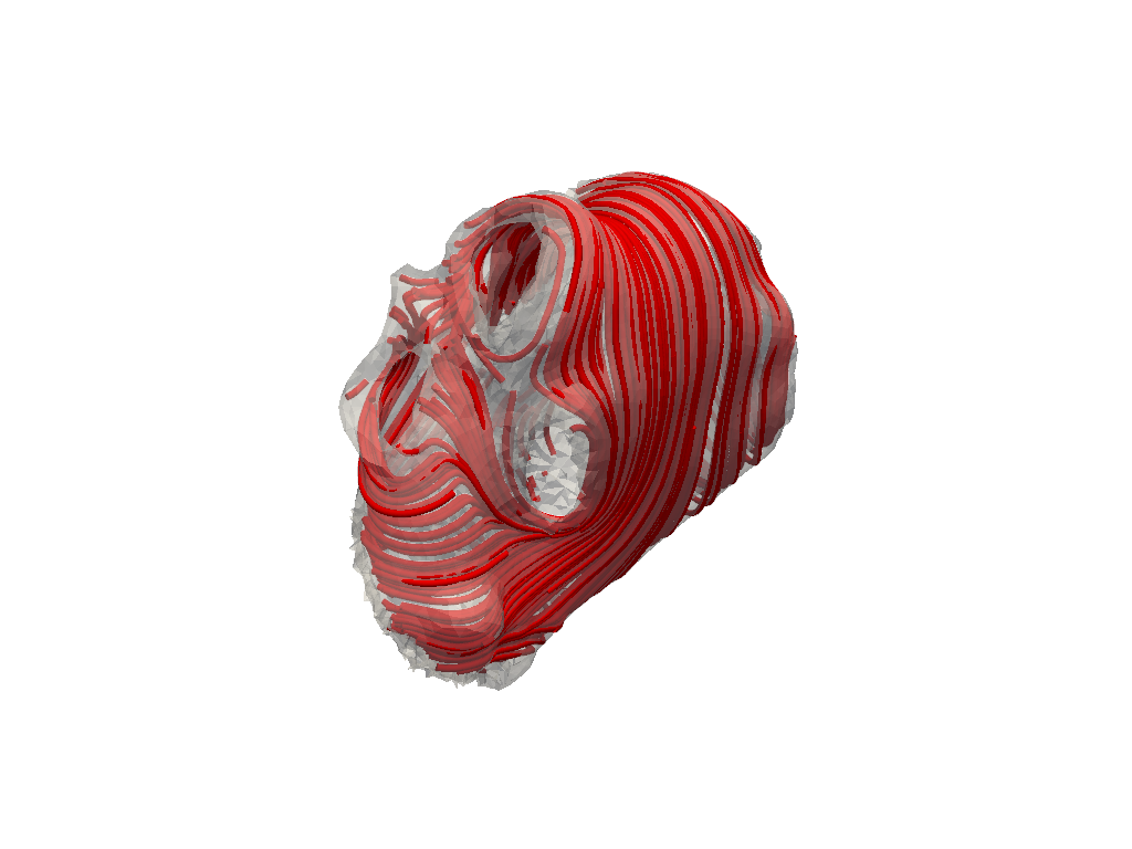
Plot left atrial fibers

# plot left atrial fibers
plotter = pv.Plotter()
mesh = la.ctp()
streamlines = mesh.streamlines(vectors="e_l", source_radius=50, n_points=5000)
tubes = streamlines.tube()
plotter.add_mesh(mesh, opacity=0.5, color="white")
plotter.add_mesh(tubes, color="red")
plotter.show()

Static Scene

Interactive Scene

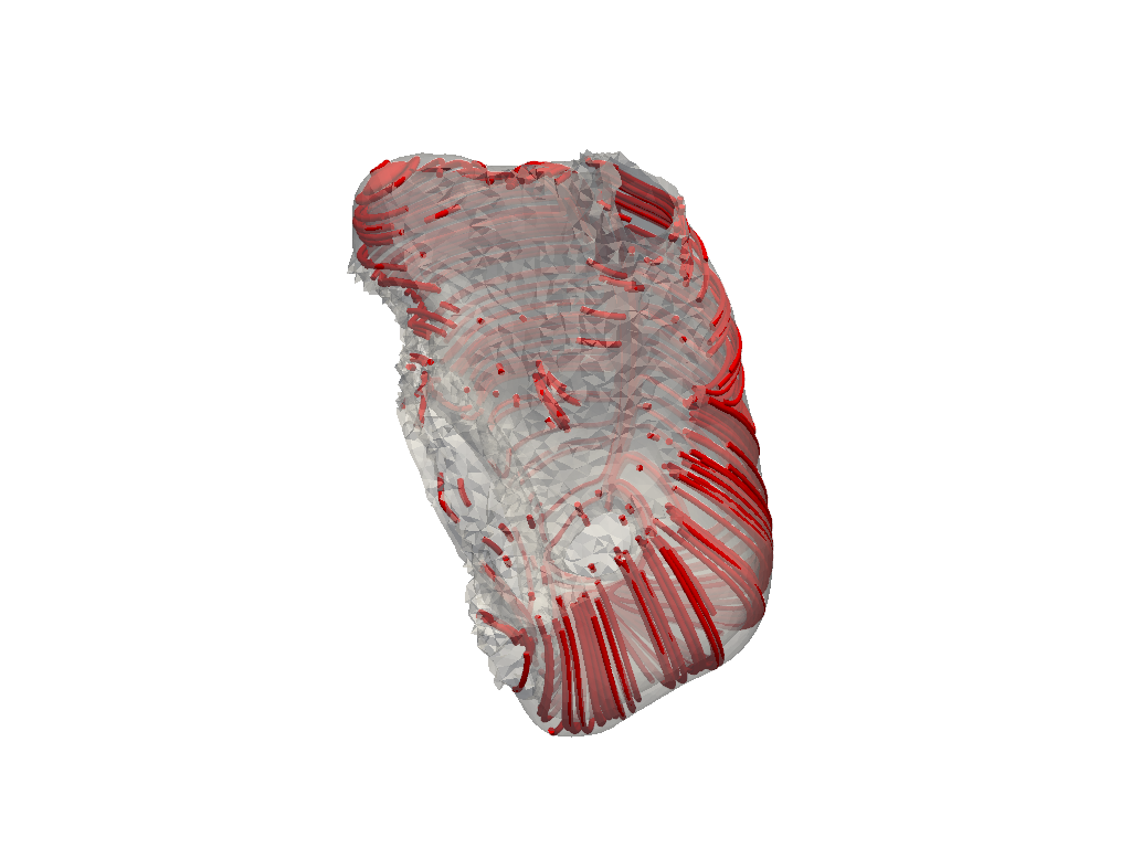
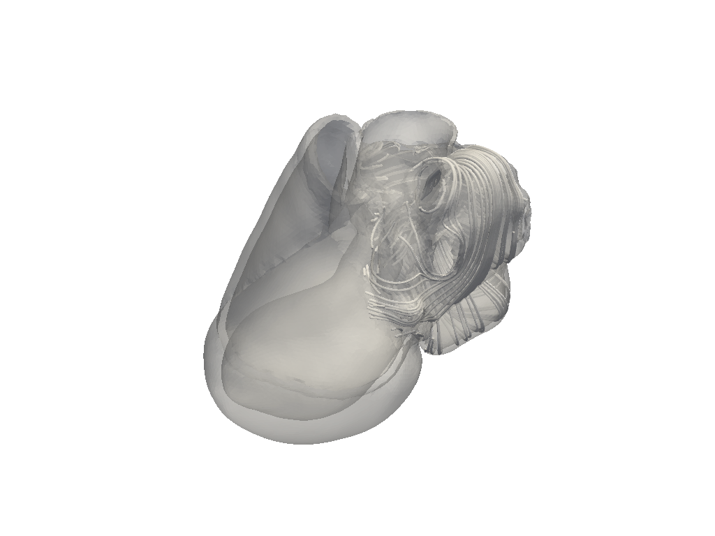
Plot right atrial fibers

# plot right atrial fibers
plotter = pv.Plotter()
mesh = ra.ctp()
streamlines = mesh.streamlines(vectors="e_l", source_radius=50, n_points=5000)
tubes = streamlines.tube()
plotter.add_mesh(mesh, opacity=0.5, color="white")
plotter.add_mesh(tubes, color="red")
plotter.show()

Static Scene

Interactive Scene

Plot full fibers on full heart model

fiber_plot = model.plot_fibers(n_seed_points=5000)

Static Scene

Interactive Scene