Run a full-heart electrophysiology simulation

This example shows how to consume a full-heart model and set it up for the main electrophysiology simulation. It loads a pre-computed heart model and computes the fiber orientation, Purkinje network, and conduction system. It then simulates the electrophysiology.

Warning

When using a standalone version of the DPF Server, you must accept the license terms. To accept these terms, you can set this environment variable:

import os
os.environ["ANSYS_DPF_ACCEPT_LA"] = "Y"

Perform the required imports

Import the required modules and set relevant paths, including that of the working directory, heart model, and LS-DYNA executable file.

import os
from pathlib import Path

from ansys.health.heart.examples import get_preprocessed_fullheart
import ansys.health.heart.models as models
from ansys.health.heart.simulator import DynaSettings, EPSimulator

# Set the working directory and path to the model. This example assumes that there is a

workdir = Path.home() / "pyansys-heart" / "downloads" / "Rodero2021" / "01" / "FullHeart"
path_to_model, path_to_partinfo, _ = get_preprocessed_fullheart(resolution="2.0mm")

Load the full-heart model

Load the full-heart model.

model: models.FullHeart = models.HeartModel.load_model(
    path_to_model, path_to_partinfo, working_directory=workdir
)

# Save the model.
model.mesh.save(os.path.join(model.workdir, "simulation_model.vtu"))

Instantiate the simulator

Instantiate the simulator and define settings.

Note

The DynaSettings object supports several LS-DYNA versions and platforms, including smp, intempi, msmpi, windows, linux, and wsl. Choose the one that works for your setup.

# Specify the LS-DYNA path. (The last tested working version is ``intelmpi-linux-DEV-106117``.)
lsdyna_path = r"ls-dyna_msmpi.exe"

# Instantiate LS-DYNA settings.
dyna_settings = DynaSettings(
    lsdyna_path=lsdyna_path, dynatype="intelmpi", num_cpus=4, platform="windows"
)

# Instantiate the simulator, modifying options as necessary.
simulator = EPSimulator(
    model=model,
    dyna_settings=dyna_settings,
    simulation_directory=os.path.join(workdir, "simulation-EP"),
)

Load simulation settings

Load the default settings.

simulator.settings.load_defaults()

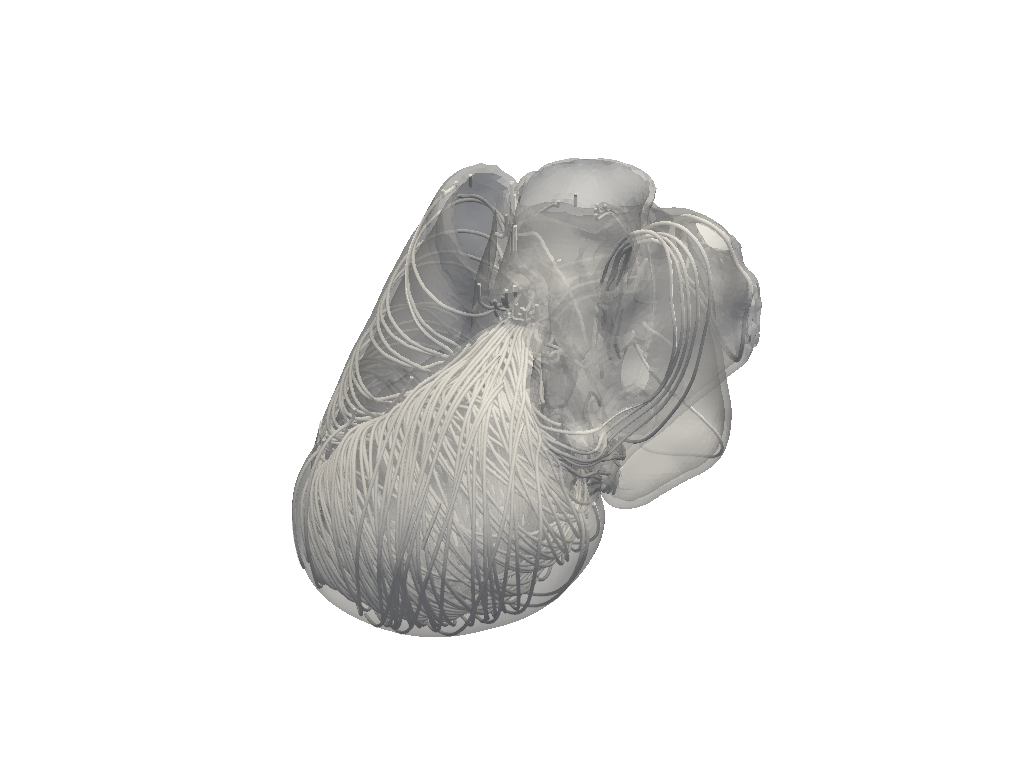
Compute fiber orientation

Compute fiber orientation and plot the fibers on the entire model.

# Compute ventricular fibers.
simulator.compute_fibers(method="D-RBM")

# Compute atrial fibers.
simulator.model.right_atrium.active = True
simulator.model.left_atrium.active = True
simulator.model.right_atrium.fiber = True
simulator.model.left_atrium.fiber = True
simulator.compute_left_atrial_fiber()
simulator.compute_right_atrial_fiber(appendage=[39, 29, 98])
simulator.model.plot_fibers(n_seed_points=1000)

Static Scene

Interactive Scene

<pyvista.plotting.plotter.Plotter object at 0x0000025804F47090>

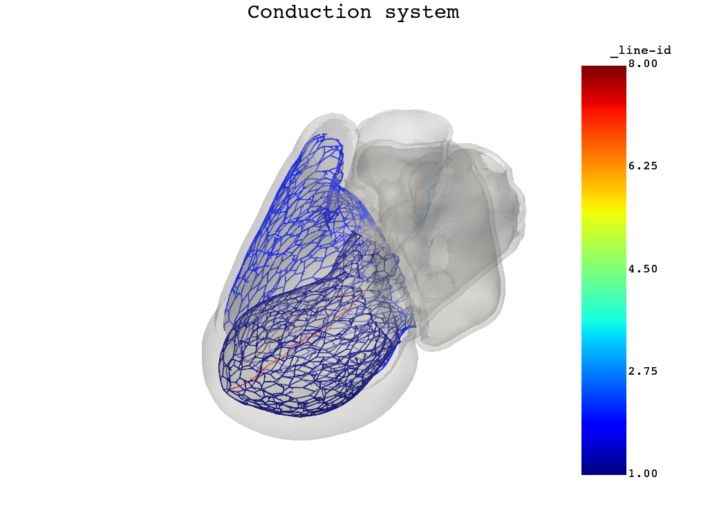
Compute the conduction system

Compute the conduction system and Purkinje network, and then visualize the results. The action potential propagates faster through this system compared to the rest of the model.

simulator.compute_purkinje()

# By calling this method, stimulation is at the atrioventricular node.
# If you do not call this method, the two apex regions of the ventricles are stimulated.
simulator.compute_conduction_system()

simulator.model.plot_purkinje()

Static Scene

Interactive Scene

Start the main simulation

Start the main electrophysiology simulation. This uses the previously computed fiber orientation and Purkinje network to set up and run the LS-DYNA model.

# Compute the Eikonal solution. This only computes the activation time.
simulator.settings.electrophysiology.analysis.solvertype = "ReactionEikonal"
simulator.simulate(folder_name="main-ep-ReactionEikonal")