Run a full-heart EP mechanics simulation

This example shows how to consume a full-heart model and set it up for a coupled electromechanical simulation.

Warning

When using a standalone version of the DPF Server, you must accept the license terms. To accept these terms, you can set this environment variable:

import os
os.environ["ANSYS_DPF_ACCEPT_LA"] = "Y"

Perform the required imports

Import the required modules.

import os
from pathlib import Path

from pint import Quantity

from ansys.health.heart.examples import get_preprocessed_fullheart
import ansys.health.heart.models as models
from ansys.health.heart.settings.material.ep_material import EPMaterial
from ansys.health.heart.settings.material.material import ISO, Mat295
from ansys.health.heart.simulator import DynaSettings, EPMechanicsSimulator

Set the required paths

Set the working directory and path to the model.

# Get the path to a preprocessed full-heart model.
path_to_model, path_to_partinfo, _ = get_preprocessed_fullheart(resolution="2.0mm")

# Set the working directory.
workdir = Path.home() / "pyansys-heart" / "downloads" / "Rodero2021" / "01" / "FullHeart"

Load the full-heart model

# Load the full-heart model.
model: models.FullHeart = models.FullHeart(working_directory=workdir)
model.load_model_from_mesh(path_to_model, path_to_partinfo)

Instantiate the simulator

# Create and instantiate a DYNA settings object. Modify where necessary.
lsdyna_path = r"your_dyna_exe"
dyna_settings = DynaSettings(
    lsdyna_path=lsdyna_path, dynatype="intelmpi", platform="wsl", num_cpus=4
)

# Instantiate the simulator.
simulator = EPMechanicsSimulator(
    model=model,
    dyna_settings=dyna_settings,
    simulation_directory=os.path.join(workdir, "ep-mechanics"),
)

# Load default simulation settings.
simulator.settings.load_defaults()

Compute the fiber orientation

# Compute fiber orientation in the ventricles and atria.
simulator.compute_fibers()
simulator.compute_left_atrial_fiber()
simulator.compute_right_atrial_fiber(appendage=[39, 29, 98])

# Switch the atria to active.
simulator.model.left_atrium.fiber = True
simulator.model.left_atrium.active = True

simulator.model.right_atrium.fiber = True
simulator.model.right_atrium.active = True

Set up the simulation for the mechanical simulations

# Extract elements around atrial caps and assign as a passive material.
ring = simulator.model.create_atrial_stiff_ring(radius=5)

# Assign a material that is stiffer than the surrounding material.
stiff_iso = Mat295(rho=0.001, iso=ISO(itype=-1, beta=2, kappa=10, mu1=0.1, alpha1=2))
ring.meca_material = stiff_iso

# Assign the default EP material
ring.ep_material = EPMaterial.Active()

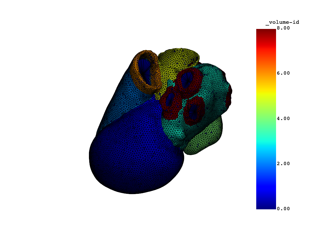
# plot the mesh
simulator.model.plot_mesh()

# Compute UHCs (Universal Heart Coordinates).
simulator.compute_uhc()

# Extract elements close to the valves and assign these a passive material.
simulator.model.create_stiff_ventricle_base(stiff_material=stiff_iso)

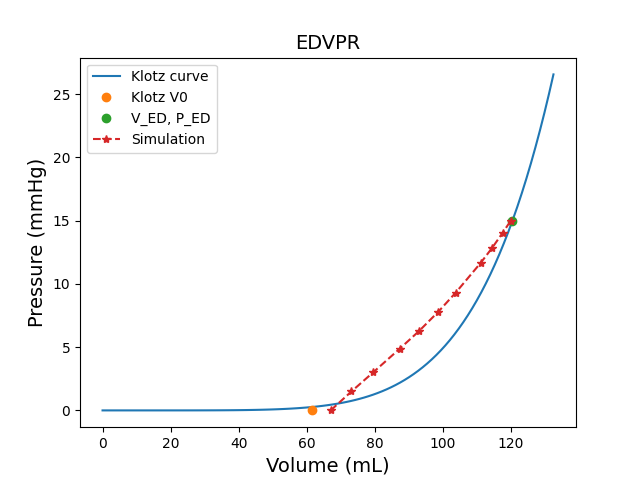
# Compute the stress-free configuration.
simulator.compute_stress_free_configuration(overwrite=True)

Static Scene

Interactive Scene

Note

Computing the stress-free configuration is required since the geometry is imaged at end-of-diastole. The compute_stress_free_configuration() method runs a sequence of static simulations to estimate the stress-free state of the model and the initial stresses present. This step is computationally expensive and can take relatively long. You can consider reusing earlier runs by setting the overwrite flag to False. This reuses the results of the previous run.

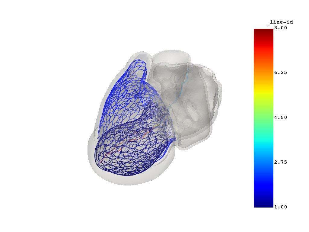
Compute a conduction system

# Compute the conduction system.
simulator.compute_purkinje()

# Use landmarks to compute the rest of the conduction system.
simulator.compute_conduction_system()

# Plot the computed conduction system.
simulator.model.plot_purkinje()

Static Scene

Interactive Scene

Start the main simulation

Set the simulation end time and frequency of output files.

simulator.settings.mechanics.analysis.end_time = Quantity(800, "ms")
simulator.settings.mechanics.analysis.dt_d3plot = Quantity(10, "ms")

# Save the model to a file.
simulator.model.save_model(os.path.join(workdir, "heart_fib_beam.vtu"))

Note

A constant pressure is prescribed to the atria. No circulation system is coupled with the atria.

# Use the ReactionEikonal solver for the electrophysiology simulation.
simulator.settings.electrophysiology.analysis.solvertype = "ReactionEikonal"

# Start main simulation. The ``auto_post`` option is set to ``False`` to avoid
# automatic postprocessing.
simulator.simulate(auto_post=False)

Note

The ReactionEikonal solver is suitable for coarse meshes and is included here for demonstration purposes. However, it currently supports only a single cardiac cycle. To simulate multiple cardiac cycles, use the Monodomain solver, which requires a fine mesh and small time step size.

Visualize and animate results LS-PrePost